Visualizations#
Tensorboard visuals#
- monai.visualize.img2tensorboard.add_animated_gif(writer, tag, image_tensor, max_out=3, frame_dim=-3, scale_factor=1.0, global_step=None)[source]#
Creates an animated gif out of an image tensor in ‘CHWD’ format and writes it with SummaryWriter.
- Parameters
writer – Tensorboard SummaryWriter to write to
tag (
str) – Data identifierimage_tensor (
Union[ndarray,Tensor]) – tensor for the image to add, expected to be in CHWD formatmax_out (
int) – maximum number of image channels to animate throughframe_dim (
int) – the dimension used as frames for GIF image, expect input data shape as CHWD, default to -3 (the first spatial dim)scale_factor (
float) – amount to multiply values by. If the image data is between 0 and 1, using 255 for this value will scale it to displayable rangeglobal_step (
Optional[int]) – Global step value to record
- Return type
None
- monai.visualize.img2tensorboard.make_animated_gif_summary(tag, image, writer=None, max_out=3, frame_dim=-3, scale_factor=1.0)[source]#
Creates an animated gif out of an image tensor in ‘CHWD’ format and returns Summary.
- Parameters
tag (
str) – Data identifierimage (
Union[ndarray,Tensor]) – The image, expected to be in CHWD formatwriter – the tensorboard writer to plot image
max_out (
int) – maximum number of image channels to animate throughframe_dim (
int) – the dimension used as frames for GIF image, expect input data shape as CHWD, default to -3 (the first spatial dim)scale_factor (
float) – amount to multiply values by. if the image data is between 0 and 1, using 255 for this value will scale it to displayable range
- Return type
Summary
- monai.visualize.img2tensorboard.plot_2d_or_3d_image(data, step, writer, index=0, max_channels=1, frame_dim=-3, max_frames=24, tag='output')[source]#
Plot 2D or 3D image on the TensorBoard, 3D image will be converted to GIF image.
Note
Plot 3D or 2D image(with more than 3 channels) as separate images. And if writer is from TensorBoardX, data has 3 channels and max_channels=3, will plot as RGB video.
- Parameters
data (
Union[~NdarrayTensor,List[~NdarrayTensor]]) – target data to be plotted as image on the TensorBoard. The data is expected to have ‘NCHW[D]’ dimensions or a list of data with CHW[D] dimensions, and only plot the first in the batch.step (
int) – current step to plot in a chart.writer – specify TensorBoard or TensorBoardX SummaryWriter to plot the image.
index (
int) – plot which element in the input data batch, default is the first element.max_channels (
int) – number of channels to plot.frame_dim (
int) – if plotting 3D image as GIF, specify the dimension used as frames, expect input data shape as NCHWD, default to -3 (the first spatial dim)max_frames (
int) – if plot 3D RGB image as video in TensorBoardX, set the FPS to max_frames.tag (
str) – tag of the plotted image on TensorBoard.
- Return type
None
Class activation map#
- class monai.visualize.class_activation_maps.CAM(nn_module, target_layers, fc_layers='fc', upsampler=<function default_upsampler>, postprocessing=<function default_normalizer>)[source]#
Compute class activation map from the last fully-connected layers before the spatial pooling. This implementation is based on:
Zhou et al., Learning Deep Features for Discriminative Localization. CVPR ‘16, https://arxiv.org/abs/1512.04150
Examples
import torch

# densenet 2d
from monai.networks.nets import DenseNet121
from monai.visualize import CAM

model_2d = DenseNet121(spatial_dims=2, in_channels=1, out_channels=3)
cam = CAM(nn_module=model_2d, target_layers="class_layers.relu", fc_layers="class_layers.out")
result = cam(x=torch.rand((1, 1, 48, 64)))

# resnet 2d
from monai.networks.nets import se_resnet50
from monai.visualize import CAM

model_2d = se_resnet50(spatial_dims=2, in_channels=3, num_classes=4)
cam = CAM(nn_module=model_2d, target_layers="layer4", fc_layers="last_linear")
result = cam(x=torch.rand((2, 3, 48, 64)))
N.B.: To help select the target layer, it may be useful to list all layers:
for name, _ in model.named_modules(): print(name)
- __init__(nn_module, target_layers, fc_layers='fc', upsampler=<function default_upsampler>, postprocessing=<function default_normalizer>)[source]#
- Parameters
nn_module (
Module) – the model to be visualizedtarget_layers (
str) – name of the model layer to generate the feature map.fc_layers (
Union[str,Callable]) – a string or a callable used to get fully-connected weights to compute activation map from the target_layers (without pooling). and evaluate it at every spatial location.upsampler (
Callable) – An upsampling method to upsample the output image. Default is N dimensional linear (bilinear, trilinear, etc.) depending on num spatial dimensions of input.postprocessing (
Callable) – a callable that applies on the upsampled output image. Default is normalizing between min=1 and max=0 (i.e., largest input will become 0 and smallest input will become 1).
- compute_map(x, class_idx=None, layer_idx=-1)[source]#
Compute the actual feature map with input tensor x.
- Parameters
x – input to nn_module.
class_idx – index of the class to be visualized. Default to None (computing class_idx from argmax)
layer_idx – index of the target layer if there are multiple target layers. Defaults to -1.
- Returns
activation maps (raw outputs without upsampling/post-processing.)
- class monai.visualize.class_activation_maps.GradCAM(nn_module, target_layers, upsampler=<function default_upsampler>, postprocessing=<function default_normalizer>, register_backward=True)[source]#
Computes Gradient-weighted Class Activation Mapping (Grad-CAM). This implementation is based on:
Selvaraju et al., Grad-CAM: Visual Explanations from Deep Networks via Gradient-based Localization, https://arxiv.org/abs/1610.02391
Examples
import torch

# densenet 2d
from monai.networks.nets import DenseNet121
from monai.visualize import GradCAM

model_2d = DenseNet121(spatial_dims=2, in_channels=1, out_channels=3)
cam = GradCAM(nn_module=model_2d, target_layers="class_layers.relu")
result = cam(x=torch.rand((1, 1, 48, 64)))

# resnet 2d
from monai.networks.nets import se_resnet50
from monai.visualize import GradCAM

model_2d = se_resnet50(spatial_dims=2, in_channels=3, num_classes=4)
cam = GradCAM(nn_module=model_2d, target_layers="layer4")
result = cam(x=torch.rand((2, 3, 48, 64)))
N.B.: To help select the target layer, it may be useful to list all layers:
for name, _ in model.named_modules(): print(name)
- compute_map(x, class_idx=None, retain_graph=False, layer_idx=-1)[source]#
Compute the actual feature map with input tensor x.
- Parameters
x – input to nn_module.
class_idx – index of the class to be visualized. Default to None (computing class_idx from argmax)
layer_idx – index of the target layer if there are multiple target layers. Defaults to -1.
- Returns
activation maps (raw outputs without upsampling/post-processing.)
- class monai.visualize.class_activation_maps.GradCAMpp(nn_module, target_layers, upsampler=<function default_upsampler>, postprocessing=<function default_normalizer>, register_backward=True)[source]#
Computes Gradient-weighted Class Activation Mapping (Grad-CAM++). This implementation is based on:
Chattopadhyay et al., Grad-CAM++: Improved Visual Explanations for Deep Convolutional Networks, https://arxiv.org/abs/1710.11063
- compute_map(x, class_idx=None, retain_graph=False, layer_idx=-1)[source]#
Compute the actual feature map with input tensor x.
- Parameters
x – input to nn_module.
class_idx – index of the class to be visualized. Default to None (computing class_idx from argmax)
layer_idx – index of the target layer if there are multiple target layers. Defaults to -1.
- Returns
activation maps (raw outputs without upsampling/post-processing.)
- class monai.visualize.class_activation_maps.ModelWithHooks(nn_module, target_layer_names, register_forward=False, register_backward=False)[source]#
A model wrapper to run model forward/backward steps and storing some intermediate feature/gradient information.
- __init__(nn_module, target_layer_names, register_forward=False, register_backward=False)[source]#
- Parameters
nn_module – the model to be wrapped.
target_layer_names (
Union[str,Sequence[str]]) – the names of the layer to cache.register_forward (
bool) – whether to cache the forward pass output corresponding to target_layer_names.register_backward (
bool) – whether to cache the backward pass output corresponding to target_layer_names.
- monai.visualize.class_activation_maps.default_normalizer(x)[source]#
A linear intensity scaling by mapping the (min, max) to (1, 0). If the input data is PyTorch Tensor, the output data will be Tensor on the same device, otherwise, output data will be numpy array.
Note: This will flip magnitudes (i.e., smallest will become biggest and vice versa).
- Return type
~NdarrayTensor
Occlusion sensitivity#
- class monai.visualize.occlusion_sensitivity.OcclusionSensitivity(nn_module, pad_val=None, mask_size=15, n_batch=128, stride=1, per_channel=True, upsampler=functools.partial(<function default_upsampler>, align_corners=True), verbose=True)[source]#
This class computes the occlusion sensitivity for a model’s prediction of a given image. By occlusion sensitivity, we mean how the probability of a given prediction changes as the occluded section of an image changes. This can be useful to understand why a network is making certain decisions.
As important parts of the image are occluded, the probability of classifying the image correctly will decrease. Hence, more negative values imply the corresponding occluded volume was more important in the decision process.
Two
torch.Tensorwill be returned by the__call__method: an occlusion map and an image of the most probable class. Both images will be cropped if a bounding box used, but voxel sizes will always match the input.The occlusion map shows the inference probabilities when the corresponding part of the image is occluded. Hence, more -ve values imply that region was important in the decision process. The map will have shape
BCHW(D)N, whereNis the number of classes to be inferred by the network. Hence, the occlusion for classican be seen withmap[...,i].The most probable class is an image of the probable class when the corresponding part of the image is occluded (equivalent to
occ_map.argmax(dim=-1)).See: R. R. Selvaraju et al. Grad-CAM: Visual Explanations from Deep Networks via Gradient-based Localization. https://doi.org/10.1109/ICCV.2017.74.
Examples:
# densenet 2d
from monai.networks.nets import DenseNet121
from monai.visualize import OcclusionSensitivity

model_2d = DenseNet121(spatial_dims=2, in_channels=1, out_channels=3)
occ_sens = OcclusionSensitivity(nn_module=model_2d)
occ_map, most_probable_class = occ_sens(x=torch.rand((1, 1, 48, 64)), b_box=[-1, -1, 2, 40, 1, 62])

# densenet 3d
from monai.networks.nets import DenseNet
from monai.visualize import OcclusionSensitivity

model_3d = DenseNet(spatial_dims=3, in_channels=1, out_channels=3, init_features=2, growth_rate=2, block_config=(6,))
occ_sens = OcclusionSensitivity(nn_module=model_3d, n_batch=10, stride=3)
occ_map, most_probable_class = occ_sens(torch.rand(1, 1, 6, 6, 6), b_box=[-1, -1, 1, 3, -1, -1, -1, -1])
See also
monai.visualize.occlusion_sensitivity.OcclusionSensitivity.
- __init__(nn_module, pad_val=None, mask_size=15, n_batch=128, stride=1, per_channel=True, upsampler=functools.partial(<function default_upsampler>, align_corners=True), verbose=True)[source]#
Occlusion sensitivity constructor.
- Parameters
nn_module (
Module) – Classification model to use for inferencepad_val (
Optional[float]) – When occluding part of the image, which values should we put in the image? IfNoneis used, then the average of the image will be used.mask_size (
Union[int,Sequence]) – Size of box to be occluded, centred on the central voxel. To ensure that the occluded area is correctly centred,mask_sizeandstrideshould both be odd or even.n_batch (
int) – Number of images in a batch for inference.stride (
Union[int,Sequence]) – Stride in spatial directions for performing occlusions. Can be single value or sequence (for varying stride in the different directions). Should be >= 1. Striding in the channel direction depends on the per_channel argument.per_channel (
bool) – If True, mask_size and stride both equal 1 in the channel dimension. If False, then both mask_size equals the number of channels in the image. If True, the output image will be: [B, C, H, W, D, num_seg_classes]. Else, will be [B, 1, H, W, D, num_seg_classes]upsampler (
Optional[Callable]) – An upsampling method to upsample the output image. Default is N-dimensional linear (bilinear, trilinear, etc.) depending on num spatial dimensions of input.verbose (
bool) – Usetqdm.trangeoutput (if available).
Utilities#
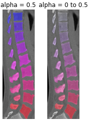
- monai.visualize.utils.blend_images(image, label, alpha=0.5, cmap='hsv', rescale_arrays=True, transparent_background=True)[source]#
Blend an image and a label. Both should have the shape CHW[D]. The image may have C==1 or 3 channels (greyscale or RGB). The label is expected to have C==1.
- Parameters
image (
Union[ndarray,Tensor]) – the input image to blend with label data.label (
Union[ndarray,Tensor]) – the input label to blend with image data.alpha (
Union[float,ndarray,Tensor]) – this specifies the weighting given to the label, where 0 is completely transparent and 1 is completely opaque. This can be given as either a single value or an array/tensor that is the same size as the input image.cmap (
str) – specify colormap in the matplotlib, default to hsv, for more details, please refer to: https://matplotlib.org/2.0.2/users/colormaps.html.rescale_arrays (
bool) – whether to rescale the array to [0, 1] first, default to True.transparent_background (
bool) – if true, any zeros in the label field will not be colored.
- monai.visualize.utils.matshow3d(volume, fig=None, title=None, figsize=(10, 10), frames_per_row=None, frame_dim=-3, channel_dim=None, vmin=None, vmax=None, every_n=1, interpolation='none', show=False, fill_value=nan, margin=1, dtype=<class 'numpy.float32'>, **kwargs)[source]#
Create a 3D volume figure as a grid of images.
- Parameters
volume – 3D volume to display. data shape can be BCHWD, CHWD or HWD. Higher dimensional arrays will be reshaped into (-1, H, W, [C]), C depends on channel_dim arg. A list of channel-first (C, H[, W, D]) arrays can also be passed in, in which case they will be displayed as a padded and stacked volume.
fig – matplotlib figure or Axes to use. If None, a new figure will be created.
title (
Optional[str]) – title of the figure.figsize – size of the figure.
frames_per_row (
Optional[int]) – number of frames to display in each row. If None, sqrt(firstdim) will be used.frame_dim (
int) – for higher dimensional arrays, which dimension from (-1, -2, -3) is moved to the -3 dimension. dim and reshape to (-1, H, W) shape to construct frames, default to -3.channel_dim (
Optional[int]) – if not None, explicitly specify the channel dimension to be transposed to the last dimensionas shape (-1, H, W, C). this can be used to plot RGB color image. if None, the channel dimension will be flattened with frame_dim and batch_dim as shape (-1, H, W). note that it can only support 3D input image. default is None.vmin – vmin for the matplotlib imshow.
vmax – vmax for the matplotlib imshow.
every_n (
int) – factor to subsample the frames so that only every n-th frame is displayed.interpolation (
str) – interpolation to use for the matplotlib matshow.show – if True, show the figure.
fill_value – value to use for the empty part of the grid.
margin (
int) – margin to use for the grid.dtype – data type of the output stacked frames.
kwargs – additional keyword arguments to matplotlib matshow and imshow.
See also
Example
>>> import numpy as np
>>> import matplotlib.pyplot as plt
>>> from monai.visualize import matshow3d
# create a figure of a 3D volume
>>> volume = np.random.rand(10, 10, 10)
>>> fig = plt.figure()
>>> matshow3d(volume, fig=fig, title="3D Volume")
>>> plt.show()
# create a figure of a list of channel-first 3D volumes
>>> volumes = [np.random.rand(1, 10, 10, 10), np.random.rand(1, 10, 10, 10)]
>>> fig = plt.figure()
>>> matshow3d(volumes, fig=fig, title="List of Volumes")
>>> plt.show()